GUI
With the GUI tool you can
visualize channels
compare channels from multiple files in the same plot
see channel, conversion and source metadata as stored in the MDF file
access library functionality for single files (convert, export, cut, filter, resample, scramble) and multiple files (concatenate, stack)
After you pip install asammdf using pip install asammdf[gui] there will be a new script called asammdf.exe in the python_installation_folder\Scripts folder.
The following dependencies are required by the GUI
PyQt5
pyqtgraph
General shortcuts
Shortcut |
Action |
Description |
|---|---|---|
F1 |
Help |
Opens this online help page |
F2 |
Create plot |
Create a new Plot window using the checked channels from the selection tree |
F3 |
Create numeric |
Create a new Numeric window using the checked channels from the selection tree |
F4 |
Create tabular |
Create a new Tabular window using the checked channels from the selection tree |
F11 |
Toggle fullscreen |
In the single files mode will display the current opened file in full screen |
Ctrl+O |
Open file(s) |
Single files
The Single files page is used to open several files individually for visualization and processing (for example exporting to csv or hdf5).
Layout elements
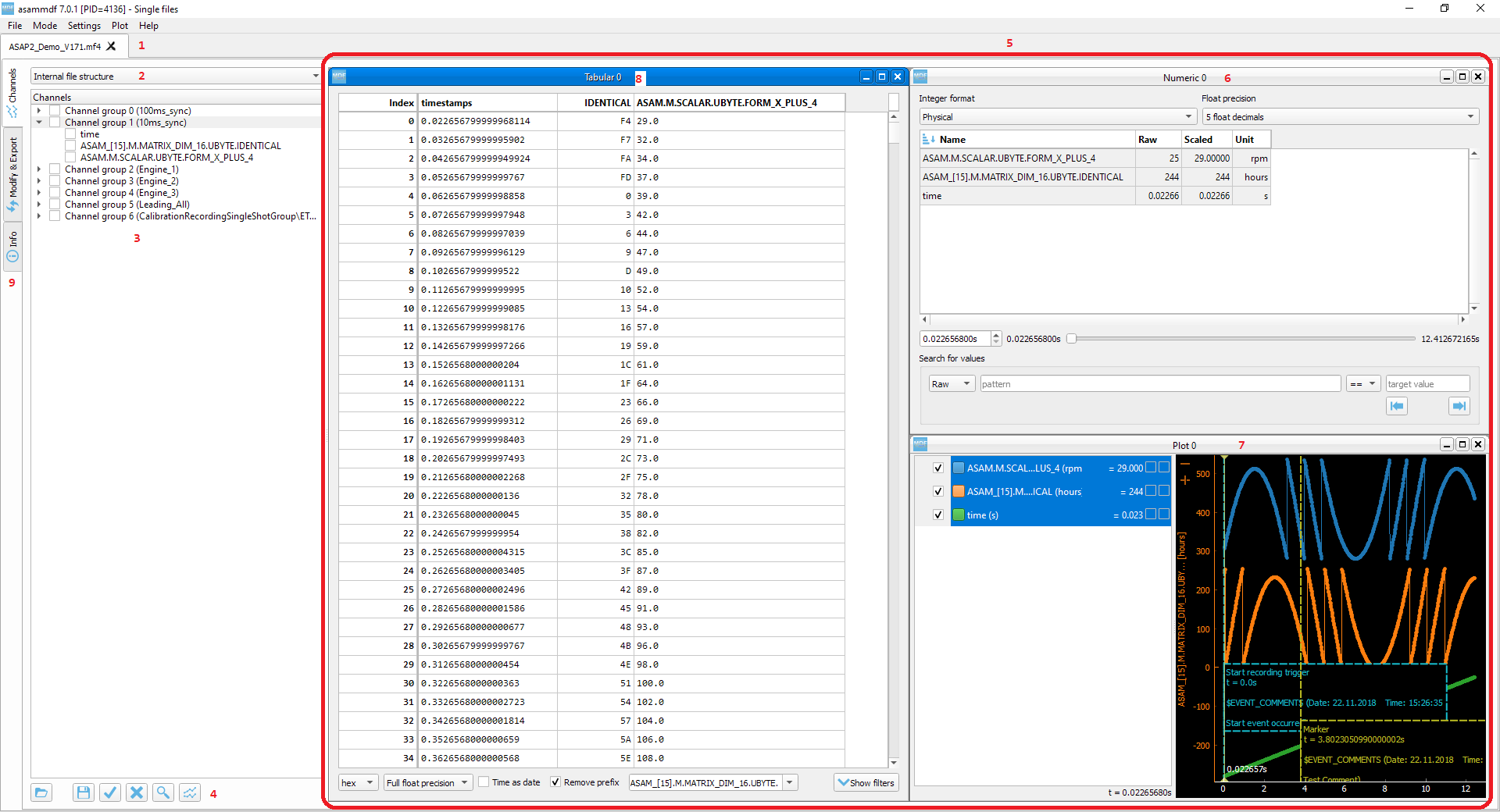
Opened files tabs
Channel tree display mode
Complete channels tree
Command buttons
Windows area
Numeric window
Plot window
Tabular window
File operations
1. Opened files tabs
In the single files mode, you can open multiple files in parallel. The tab names have the title set to the short file name, and the complete file path can be seen as the tab tool-tip.
There is no restriction, so the same file can be opened several times.
2. Channel tree display mode
The channel tree can be displayed in three ways
as a naturally sorted list
grouped using the internal file structure
only the selected channels
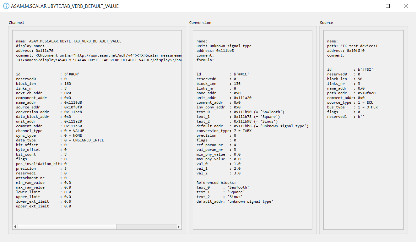
3. Complete channels tree
This tree contains all the channels found in the measurement.
Double clicking a channel name will display a pop-up window with the channel information (CNBLOCK, CCBLOCK and SIBLOCK/CEBLOCK)
Only the channels that are checked in the channels tree will be selected for plotting when the Create window button is pressed. Checking or unchecking channels will not affect the current plot or sub-windows.
4. Command buttons
From left to right the buttons have the following functionality
Load configuration: restores channels tree and all sub-plot windows from a saved configuration file
Save configuration: saves all sub-windows (channels, colors, common axis and enable state) and channel tree
Select all channels: checks all channels in the channels tree
Reset selection: unchecks all channels in the channels tree
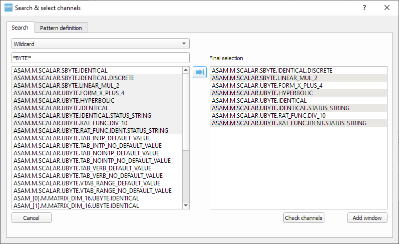
Advanced search & select: will open an advanced search dialog
the dialog can use wildcard and regex patterns
multiple channels can be selected, and thus checked in the channels tree
in the “Pattern based window” tab the user can define a pattern that will be used to filter out the channels from the measurement file, and as a second filtering step some condition can be used based on the channels values. This information will be saved in the window configuration. The pattern based windows can be easily recognized by the title bar icon
the keyboard shortcut
Ctrl+Fcan also be used to bring up the search dialog
Create window: generates a new window (Numeric, Plot, Tabular, GPS, CAN/LIN/FlexRay Bus Trace) based on the current checked channels from the channels tree. If sub-windows are disabled in the settings then the current window is replaced by the new plot. If sub-windows are enabled then a new sub-plot will be added, and the already existing sub-windows will not be affected. The same channel can be used in multiple sub-windows.
5. Windows area
If sub-windows are enabled then multiple plots can be used. The sub-windows can be re-arranged using drag & drop.
6. Numeric window
Numeric windows can handle a lot more channels than plot windows. You can use a numeric window to see the channel values at certain time stamps, and to search for certain channel values.
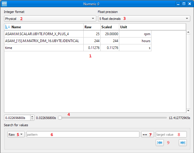
display area: here we can see the instantaneous signal values. The raw and scaled values are shown for each signal. Double clicking a column header will toggle the sorting on that column.
integer format: choose between physical, hex and binary format.
float decimals: choose the precision used for float display
timestamp selection: use the input box or the slider to adjust the timestamp
signal values search mode: choose between raw and scaled signal samples when searching for a certain value
signal name pattern: use a wildcard pattern to select the signals that will be used for value searching
operator: operator that will be used for the search
target value: search target value
direction: timebase direction for searching the values
Double clicking a row will bring up the range editor for associated signal.
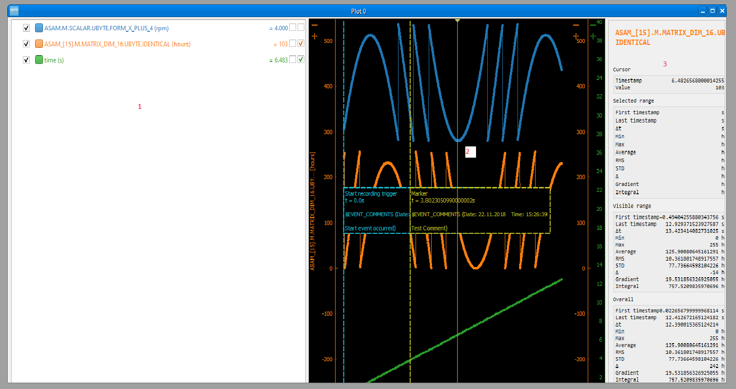
7. Plot window
Plot windows are used to graphically display the channel samples.
pyqtgraph is used for the plots; to get the best performance consider the following tips.
limit the number of channels: plotting hundreds of channels can get really slow
disabling dots will make the plots a lot more responsive
The Plot window has three section
1. signal selection tree
2. graphical area
3. signal statistics panel (toggled using the M keyboard shortcut)
Each signal item from the signal selection tree has five elements
display enable checkbox
color select button
channel name and unit label
channel value label [4]
common axis checkbox
individual axis checkbox [5]
The user can also create channel groups in the selection tree. Simple channel groups are only used for grouping signals. Pattern based channel groups can be used to filter signals based on the name or samples values.
The selection tree has an extended context menu accessible using the right mouse click.
Double clicking an item will open a range editor dialog, similar to the Numeric window range editor.
The initial graphics are view will have all the signal homed-in (see the H keyboard shortcut). The user is free to use the mouse to interact with the graphics area (zoom, pan).
The cursor is toggled using the C keyboard shortcut, and with it the channel values will be displayed for each item in the Selected channels list. The cursor can also be invoked by clicking the plot area.
Using the R keyboard shortcut will toggle the range, and with it the channel values will be displayed for each item in the Selected channels list. When the range is enabled, using the H keyboard shortcut will not home to the whole time range, but instead will use the range time interval.
The Ctrl+H, Ctrl+B and Ctrl+P keyboard shortcuts will
change the axis values for integer channels to hex, bin or physical mode
change the channel value display mode for each integer channel item in the Signal selection tree
The Alt+R and Alt+S keyboard shortcuts will switch between the raw and scaled signal samples.
Each vertical axis width can be modified using the + and - buttons.
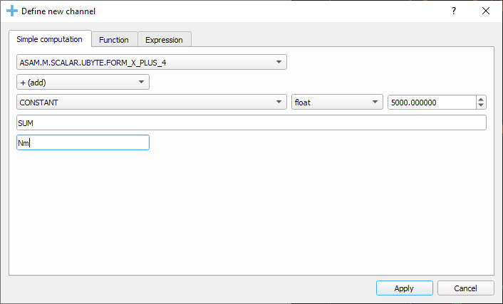
You can insert new computed channels by pressing the insert key. This will allow either to compute basic operations using the plot channels, to apply a function on one of the plot channels, or to specify a simple expression than uses multiple signals from the Plot window.
The currently active plot’s channels can be saved to a new file by pressing Ctrl+S. The channels from all sub-windows can be saved to a new file by pressing Ctrl+Shift+S.
The sub-windows can be tiled as a grid, vertically or horizontally (see the keyboard shortcuts).
8. Tabular window
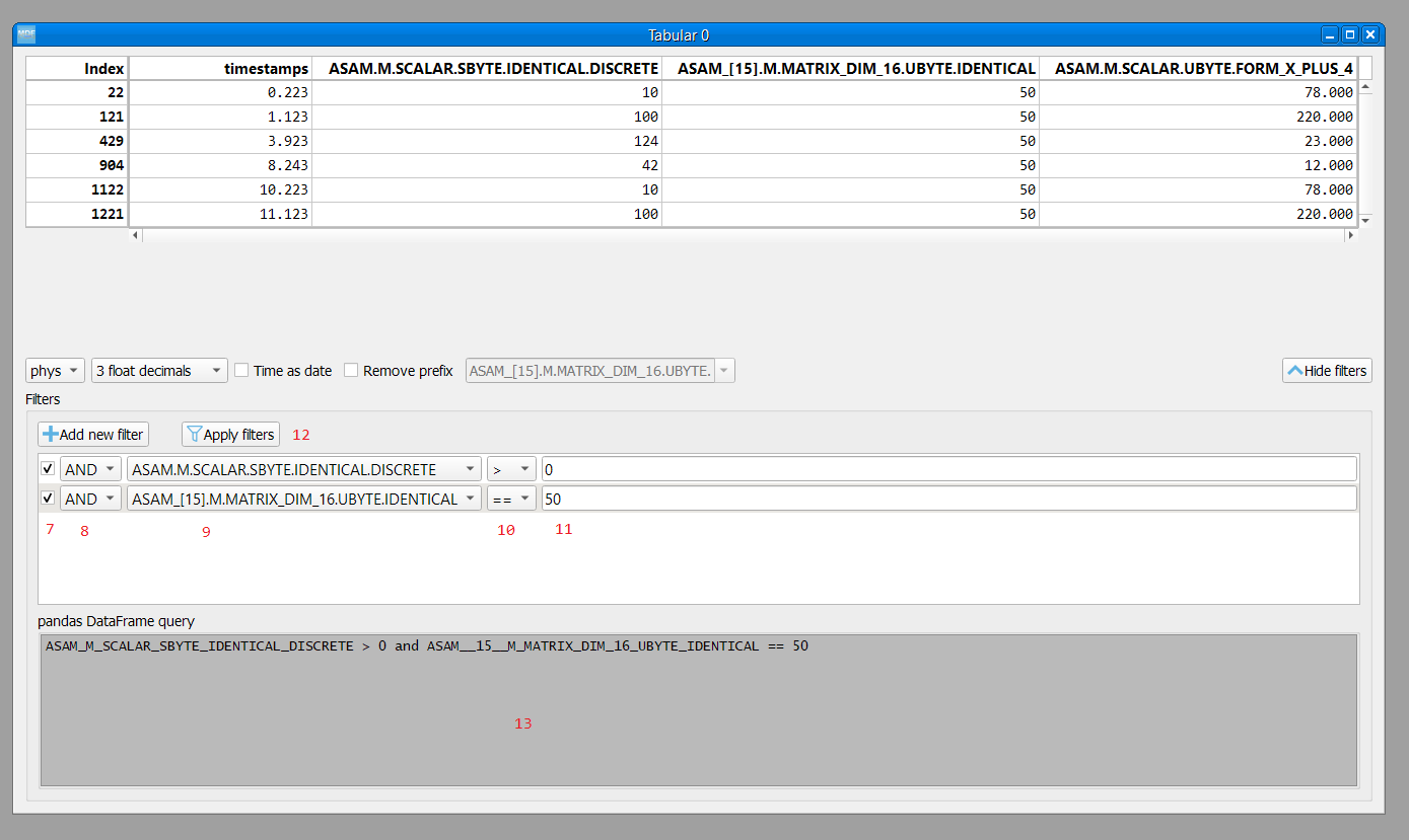
The tabular window is very similar to an Excel/CSV sheet. The most powerful feature of this window is that multiple filters can be defined for the signals values.
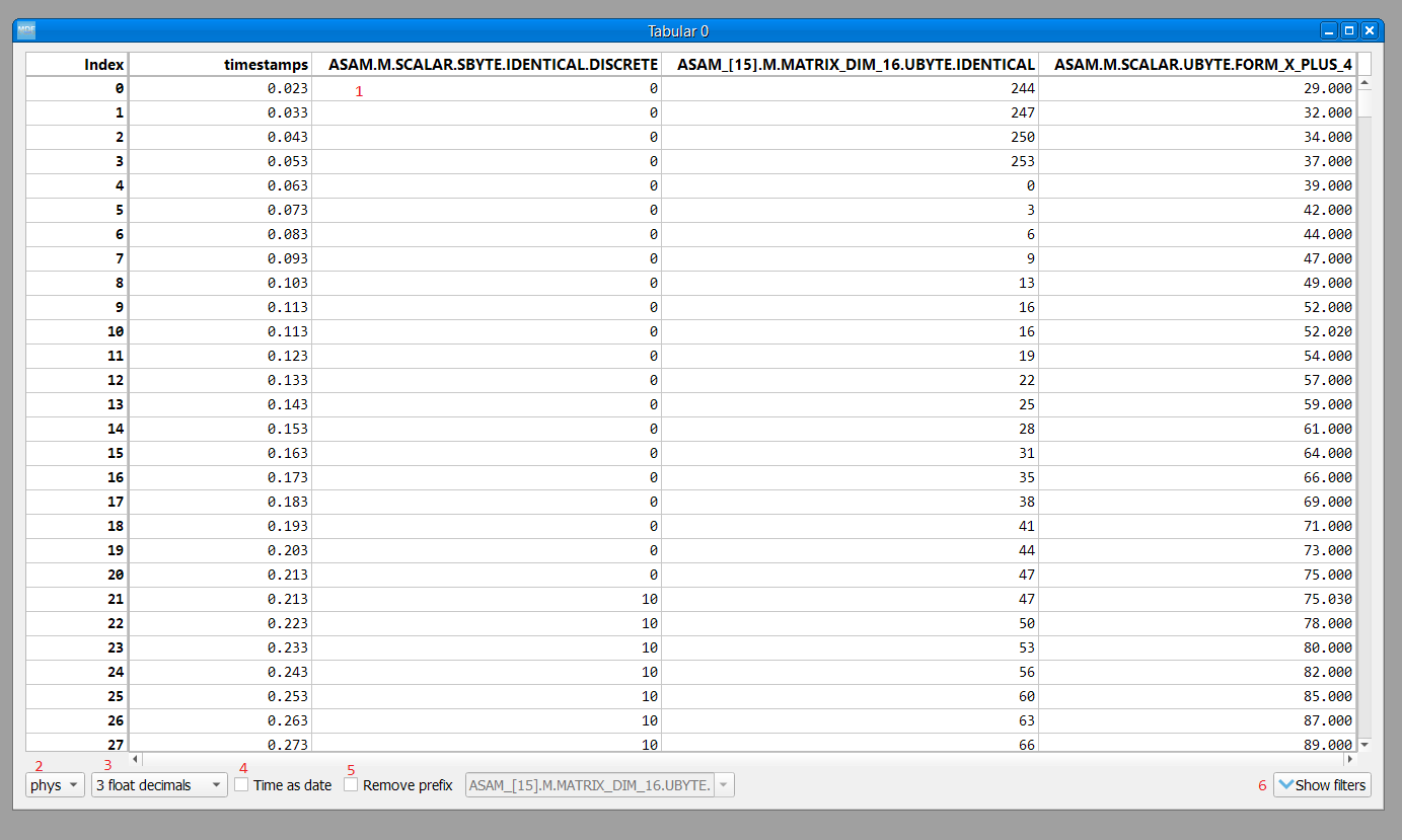
The tabular window has the following elements:
display area: here we can see the signal values. The raw and scaled values are shown for each signal. Right clicking a column header will show a pop-up window for controlling the sorting, defining signal ranges and adjusting the columns width.
integer format: choose between physical, hex and binary format.
float decimals: choose the precision used for float display
timestamp format: use the input box or the slider to adjust the timestamp display as float value or as datetime value
remove prefix: remove column names prefix; avoids unnecessary large column widths
toggle filters view: toggle the visibility of the filters (better vertical space if filters are not used)
filter enable
filter logical relation
filtering signal
filter operator
target value for filtering
apply filters: the actual filtering is done only after pressing the button. The user can modify the existing filters without changing the tabular view.
query: the Tabular window used a pandas dataframe as backend. The filtering is done by performing a query on the dataframe.
9. File operations
There are five aspects related to the measurement file that can be accessed using the tabs:
channels: here the user can visualize the signals using the available window types
modify & export: this tab contains the tools needed for processing the measurement file. The use can filter signals, cut and resample the measurement, or export it to other file formats.
bus logging: this tab is only visible for the measurements that contain CAN or LIN bus logging. The user can decode the raw bus logging using database files (.dbc, .ldf, .arxml)
attachments: this tab is only visible if the measurement contains attachments. The user can extract the attachment and save it to a new file.
info: this tab contains an overview of the measurement file content (channel groups, file header comments, total number of channels)
10. CAN/LIN/FlexRay Bus Trace
This window types can only be created by pressing the Create window button. If the measurement
does not contain bus logging of the selected kind, then no window will be generated.
The filtering and signal ranges definition is done similar to the Tabular window.
11. Drag & Drop
Channels can be dragged and dropped between sub-windows for easier configuration. Drag and drop in the free MDI can be used to create new windows.
Batch processing
The Batch processing view is used to concatenate or stack multiple files, or to perform the same processing steps on multiple files.
Keep in mind that the order of the input files is always preserved, only the samples timestamps are influenced by the Sync using measurements timestamps checkbox.
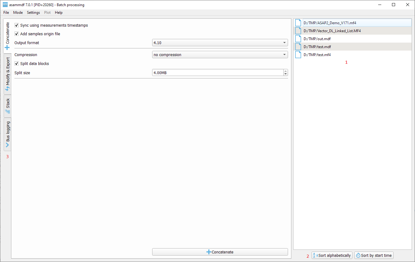
file list
file list sorting buttons
batch operations
concatenate requires input files with matching internal structure (same number of channel groups and the same set of channels in each n-th group). Each signal in the output file will be the result of concatenation of the samples from the input files
modify & export: similar to the single files view
stack will create a single measurement that will contain all the channel groups from the input files. Identically named channels will not be concatenated, they will just appear multiple times in the output file
bus logging: similar to the single files view
The files list can be rearranged in the list (1) by drag and dropping lines. Unwanted files can be deleted by selecting them and pressing the DEL key. The files order is considered from top to bottom.
Comparison
Use CTRL+F to search channels from all the opened files. The channel names are prefixed with the measurement index.
Footnotes