Functions manager view

Virtual channels (computed channels) can be defined in the Plot windows. The user will define the functions used for the virtual channels using Python language syntax; the extra rules will be described lower. After this the user can insert virtual channels in the Plot window (keyboard shortcut Ins) and will map an existing function to the virtual channel, as well as a list of alternative channel names (ASAPs) for each function argument.

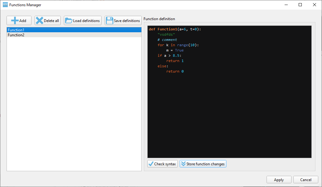
Function manager dialog

The user defined functions are associated with the display file. This means that there will be separate function managers for each opened measurement file. When a display file (.dspf) is saved by the user it will also contain the associated user defined functions. The functions manager dialog can be invoked using the keyboard shortcut F6.

Option	Description
Add	Adds a new function
Delete all	Deletes all the defined functions
Load definitions	Imports definitions found in .def files
Save definitions	Saves all the define function to a new file with the extension .def
Function definition	Python language function definition
Check syntax	Check if the current function definition syntax is valid
Store function changes	Updates the definition after the user has made changes. If this is not pressed and the user switches to another function then the changes will be lost.
Apply	Accept all the changes made by the user
Cancel	Rejects all the changes made by the user

Python function rules

The user defines the functions using Python syntax; this means that the function definition must be valid in Python code.

Further more the following rules and restrictions must be followed:

• all function arguments must have default numeric values: this means that the definition def Function1(a, b, t=0) is not accepted, instead the user must provide default values such as def Function1(a=1.5, b=0, t=0)

• the last argument must be t=0: the argument t is reserved for the time stamp and must not be otherwise used by the user. This means that the definition def Function1(a=1.5, b=0) is not valid, instead the user can write something like this def Function1(a=1.5, b=0, t=0)

• always return numeric values on all the branches: Python functions automatically return None if no return is explicitly written. The user must take care that all possible code braces return numeric values.

  "this function will produce errors because not all branches have explicit return statements with numeric values"
  def Function1(a=0, t=0):
      if a > 5:
          return 1
  
  "this function will produce errors because it returns non-numeric values"
  def Function1(a=0, t=0):
      if a > 5:
          return "Activated"
      else:
          return "Disabled"
  
  "this function is OK because it has explicit return statements with numeric values"
  def Function1(a=0, t=0):
      if a > 5:
          return 1
      else:
          return 0
  

• the modules math, pandas and numpy are available inside the function as math, pd and np

• functions can be cross-referenced; one function can call another user defined function

  def Function1(a=0, t=0):
      if a > 5:
          return 1
      else:
          return 0
  
  " Function2 can call Function 1"
  def Function2(b=1, c=7, t=0):
      if b != 0:
          return Function1(c)
      else:
          return c / 2
  

Virtual channel dialog

Virtual channels can be added to Plot windows using the keyboard shortcut Ins (insert). The precondition for this is to have at least one function defined in the Functions manager.

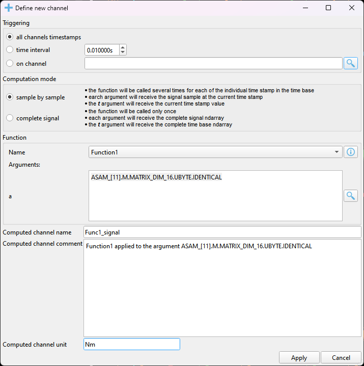
In the Define channel dialog window the user can select one of the available function, and then for each of the function’s arguments a list of alternative channel names can be filed by the user. The argument t=0 is reserved for the time-stamp and is not shown in the dialog window. The alternative names must be placed on separate lines in the text field found next to the argument name.

Option	Description
Triggering	the virtual channel samples will be calculated in the time stamps defined by the selected choice
Computation mode	the virtual channel can be computed passing the signal arguments samples by sample or passing the signal arguments directly as numpy ndarrays
Function name	select one of the available functions
Function info	displays the function definition code
Arguments	alternative channel names for each argument. In the example argument b will use the first existing ASAP from the choices MAIN_CLOCK or MAIN_CLOCK_5MS. If no alternative exist in the measurement file then the argument’s default value will be used (see the function definition)
Argument search	opens a search dialog were channel names cane be searched from the measurement file
Computed channel name	virtual channel name
Computed channel comment	virtual channel comment
Computed channel unit	virtual channel unit
Function definition	Python language function definition
Check syntax	Check if the current function definition syntax is valid
Store function changes	Updates the definition after the user has made changes. If this is not pressed and the user switches to another function then the changes will be lost.
Apply	Accept the changes and inserts the new virtual channel
Cancel	Rejects all the changes made by the user

When the computation mode is set to sample by sample the following steps are executed:

• the signals linked to the arguments are searched in the measurement file

• using the signals found in the measurement, the union of all time stamps is computed (resulting an ndarray of length N)

• all found signals are interpolated using the union time base

• the function is called N times (once for each of the N time stamps) passing the signal value for the current time stamp and the time stamp (in the t argument). The missing linked signals will be replaced by the default value specified in the function definition

• the returned value are stored and finally the resulting Signal is constructed

When the computation mode is set to complete signal the following steps are executed:

• the signals linked to the arguments are searched in the measurement file

• using the signals found in the measurement, the union of all time stamps is computed (resulting an ndarray of length N)

• all found signals are interpolated using the union time base

• the function is called only 1 time passing the complete signal ndarray’s and the union of the time stamps (in the t argument). The missing linked signals will be replaced by an ndarray of length N filled with the default value specified in the function definition

• the result Signal is constructed using the ndarray returned by the function

Example functions

Average of 3 channels

The same definition works for both sample by sample and complete signal computation modes

def average(channel1=0, channel2=-1, channel3=0, t=0):
    return (channel1 + channel2 + channel3) / 3

Channel clipping

Using sample by sample computation mode

def clip(channel1=0, t=0):
    if channel1 > 100:
        return 100
    elif channe1 < 0:
        return 0
    else:
        return channel1

Using complete signal computation mode

def clip(channel1=0, t=0):
    return np.clip(cahnnel1, 0, 100)

Grey code to decimal

The same definition works for both sample by sample and complete signal computation modes

def gray2dec(position_sensor_value=0, t=0):

    for shift in (8, 4, 2, 1):
        position_sensor_value = position_sensor_value ^ (position_sensor_value >> shift)

    return position_sensor_value

Maximum of 3 channels

Using sample by sample computation mode

def maximum(channel1=0, channel2=-1, channel3=0, t=0):
    return max(channel1, channel2, channel3)

Using complete signal computation mode

def maximum(channel1=0, channel2=-1, channel3=0, t=0):
    return np.maximum.reduce([channel1, channel2, channel3])

rpm to rad/s

The same definition works for both sample by sample and complete signal computation modes

def rpm_to_rad_per_second(speed=0, t=0):
    return 2 * np.pi * speed / 60

gradient

In the Define channel dialog the computation mode must be set to complete signal

def rpm_to_rad_per_second(speed=0, t=0):
    return np.diff(speed) / np.diff(t)

It is not possible to implement this function in the sample by sample mode because only the current samples are forwarded to the function.